Link measured data to the twin#

This tutorial continues Simulate the twin’s ECM. Your P45B twin ends that tutorial at version 4, carrying a simulated discharge. Now it meets reality: you will link the measured 1C discharge from the same About:Energy release, estimate the cell’s state from the measurement by coulomb counting, and let the twin quantify how well its own model matches the lab, ending with the comparison figure below.

As before, every output shown is from a real run (2026-08-10, battwin 0.4.0).

1. Get the measured data#

The About:Energy release does not just carry model parameters; it carries the validation measurements behind them. Download the data archive from Zenodo and pull out the test that matches our simulation, the 1C constant-current discharge at 25 °C:

curl -L -o molicel_p45b_data.zip \
  "https://zenodo.org/api/records/19052626/files/molicel_p45b_data.zip/content"
unzip molicel_p45b_data.zip MOLICEL_P45B_025degC_1C_Dch.csv

Skipping the 12 MB download

The converted result of steps 1–3, p45b-measured-1c-25degC.bdf.csv, ships in examples/p45b/ — copy it into your working directory and jump to step 4.

The data is CC-BY-4.0: cite the dataset DOI (10.5281/zenodo.19052626) if you use it beyond this tutorial. The test matrix and methods behind these measurements are described in the release’s accompanying paper, Dickinson et al. (SSRN 6861858), §4 and §6.

2. Look at what you downloaded#

$ head -2 MOLICEL_P45B_025degC_1C_Dch.csv
t_s,I_exp_A,V_exp_V,T_exp_degC,I_sim_A,V_sim_V,SOC_sim,E_OCV_V,T_sim_degC,Q_sim_W
0,-0.0028854520177433,4.18726253105995,25,-0.0028854520177433,4.18750973261517,1,4.18752999592138,25,3.08356765907969e-05

Two things to notice. First, the file mixes measurement columns (*_exp_*) with About:Energy’s own model output (*_sim_*); we want only the measurement — the twin already has its own simulation. Second, the measured current is negative during discharge, which happens to match the BDF sign convention (positive = charging) already, so no sign flip is needed. Checking that is a step you should never skip when ingesting someone else’s data; cyclers disagree about signs constantly.

3. Convert to BDF column naming#

Save as convert_measured.py:

import csv

with open("MOLICEL_P45B_025degC_1C_Dch.csv", encoding="utf-8-sig", newline="") as f:
    rows = list(csv.DictReader(f))

with open("p45b-measured-1c-25degC.bdf.csv", "w", newline="", encoding="utf-8") as f:
    writer = csv.writer(f)
    writer.writerow(["test_time_second", "current_ampere", "voltage_volt",
                     "surface_temperature_celsius"])
    for r in rows:
        writer.writerow([r["t_s"], r["I_exp_A"], r["V_exp_V"], r["T_exp_degC"]])

t = [float(r["t_s"]) for r in rows]
i = [float(r["I_exp_A"]) for r in rows]
v = [float(r["V_exp_V"]) for r in rows]
print(f"{len(rows)} samples over {t[-1]:.0f} s")
print(f"current: {min(i):.2f} to {max(i):.2f} A (negative = discharging, BDF convention)")
print(f"voltage: {v[0]:.3f} V -> {v[-1]:.3f} V")

$ python convert_measured.py
3433 samples over 3434 s
current: -4.50 to -0.00 A (negative = discharging, BDF convention)
voltage: 4.187 V -> 2.499 V

Compare that last line with the simulation from the previous tutorial: the measured cell reached the 2.5 V cut-off at 3434 s, while the simulated one ran the full 3600 s and stopped at its SoC floor at 2.62 V. Keep that discrepancy in mind; it comes back in step 6. (In production, this measure-and-convert step is battfeed’s job — it writes BDF files straight from the cycler.)

4. Link the measurement as version 5#

Save as link_data.py:

from battwin import DataLink, load, save

v4 = load("p45b.v4.twin.json")
v5 = v4.next_version(
    data=list(v4.data) + [
        DataLink(
            kind="bdf",
            uri="p45b-measured-1c-25degC.bdf.csv",
            role="characterization",
            description="Measured 1C CC discharge at 25 degC, About:Energy validation "
            "data release (Zenodo 10.5281/zenodo.19052626, CC-BY-4.0), converted to "
            "BDF column naming; measurement columns only",
        )
    ]
)
save(v5, "p45b.v5.twin.json")
print(v5.version.number, v5.version.changed)
print("data links:", [(d.role, d.uri) for d in v5.data])

Note list(v4.data) + [...]: when a new version updates a section, it replaces that section wholesale — there is no merging. If you passed only the new link, the simulation link from version 4 would vanish from version 5. Carrying the existing links forward is your job; the previous tutorial did this too, quietly.

$ python link_data.py
5 ['data']
data links: [('simulation', 'p45b-sim-1c-25degC.bdf.csv'), ('characterization', 'p45b-measured-1c-25degC.bdf.csv')]

$ battwin validate p45b.v5.twin.json
ok       p45b.v5.twin.json

$ battwin diff p45b.v4.twin.json p45b.v5.twin.json
versions: 4 -> 5
changed sections: data
version chain: intact (b.previous == hash(a))

The envelope links the dataset by URI and describes its role and provenance; it does not embed the 168 kB of samples. Data stays in data files, the twin stays a small document.

5. Estimate state from the measurement#

A linked dataset can now feed a state estimate. Coulomb counting is the textbook method: integrate current over time to get the charge actually delivered. Save as estimate_state.py:

import csv
from datetime import datetime, timezone

from battwin import StateSnapshot, load, save

with open("p45b-measured-1c-25degC.bdf.csv", encoding="utf-8", newline="") as f:
    rows = [(float(r["test_time_second"]), float(r["current_ampere"]))
            for r in csv.DictReader(f)]

# Coulomb counting: integrate current over time (trapezoid rule).
# BDF sign is positive = charging, so a discharge integrates negative.
charge_as = sum(
    0.5 * (i0 + i1) * (t1 - t0)
    for (t0, i0), (t1, i1) in zip(rows, rows[1:])
)
discharged_ah = -charge_as / 3600.0
nominal_ah = 4.5
soh = discharged_ah / nominal_ah

print(f"discharged capacity: {discharged_ah:.3f} Ah (nominal {nominal_ah} Ah)")
print(f"state of health: {soh:.3f}")

v5 = load("p45b.v5.twin.json")
v6 = v5.next_version(
    state=StateSnapshot(
        as_of=datetime.now(timezone.utc),
        state_of_charge=0.0,
        state_of_health=round(soh, 3),
        method="coulomb_counting over measured 1C discharge to 2.5 V cut-off",
        source_data="p45b-measured-1c-25degC.bdf.csv",
    )
)
save(v6, "p45b.v6.twin.json")
print(v6.version.number, v6.version.changed)

$ python estimate_state.py
discharged capacity: 4.292 Ah (nominal 4.5 Ah)
state of health: 0.954
6 ['state']

The estimate carries its own accountability: method says how it was computed and source_data names the linked dataset it came from, so anyone holding the twin can re-derive the number.

Is 95.4% the “real” SoH?

Delivered capacity is rate- and cut-off-dependent: a 1C discharge to 2.5 V delivers less than a slow one, so this figure slightly understates the cell’s low-rate capacity. The release also contains C/30 tests (*_Co30_*.csv), which would be the better SoH basis. The point here is the mechanism — a defensible, source-linked estimate — not the last word on this cell.

6. Ask the twin how good its model is#

The twin now links a simulation and a measurement of the same protocol, so comparing them is a few lines. Save as compare.py:

import csv
from bisect import bisect_left


def read(path):
    with open(path, encoding="utf-8", newline="") as f:
        rows = list(csv.DictReader(f))
    return ([float(r["test_time_second"]) for r in rows],
            [float(r["voltage_volt"]) for r in rows])


def interp(x, xs, ys):
    k = bisect_left(xs, x)
    if k == 0 or k >= len(xs):
        return ys[0] if k == 0 else ys[-1]
    f = (x - xs[k - 1]) / (xs[k] - xs[k - 1])
    return ys[k - 1] + f * (ys[k] - ys[k - 1])


mt, mv = read("p45b-measured-1c-25degC.bdf.csv")
st, sv = read("p45b-sim-1c-25degC.bdf.csv")

errors = [interp(t, st, sv) - v for t, v in zip(mt, mv)]
rmse = (sum(e * e for e in errors) / len(errors)) ** 0.5
mae = sum(abs(e) for e in errors) / len(errors)
print(f"voltage error, simulated vs measured: RMSE {rmse*1000:.1f} mV, MAE {mae*1000:.1f} mV")

$ python compare.py
voltage error, simulated vs measured: RMSE 76.9 mV, MAE 53.6 mV

Line chart of terminal voltage against time for the 1C discharge at 25 degrees Celsius. The measured curve and the twin's simulated curve track each other closely for most of the hour, with the simulation reading slightly high. Near the end of discharge they diverge, the measured cell reaching the 2.5 volt cut-off at about 57 minutes while the simulation continues to 60 minutes and stops at 2.62 volts. 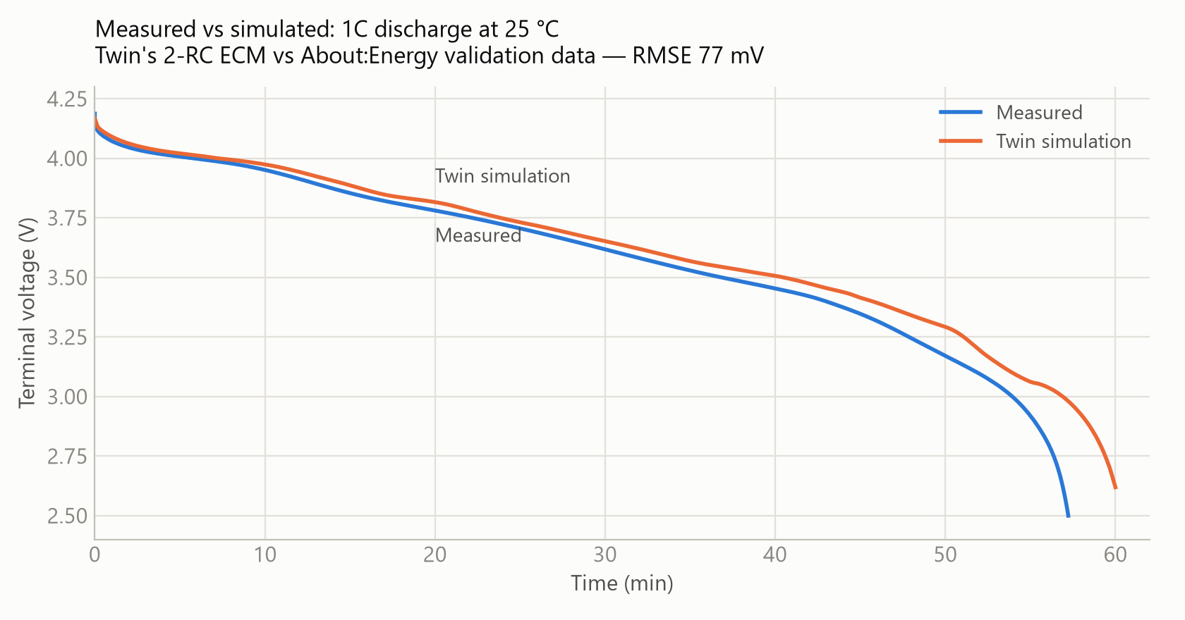— Measured vs simulated terminal voltage for the same 1C discharge, plotted from the twin’s two linked data files. RMSE 77 mV over the measured hour.#

The curves track within tens of millivolts for most of the discharge, and then diverge exactly where you would expect a simplified model to struggle: at the end-of-discharge knee, where the averaged OCV (remember the hysteresis warning from the previous tutorial) and the model’s SoC floor bite. The measured cell hits 2.5 V at 57 minutes with 4.29 Ah delivered; the simulation coasts to its SoC floor at 60 minutes. This is the quiet payoff of linking measured data: the twin becomes its own model critic, with the evidence attached.

For calibration of that criticism: Dickinson et al. report 17.3 mV RMS error for this very test, but under their metric (down to 10% SoC) and with the full hysteresis model. Most of the gap between their 17.3 mV and our 77 mV is battwin’s averaged-OCV projection — the branch half-gap averages ~29 mV over that SoC range on this SiOx-anode cell — plus the sub-10%-SoC region their metric excludes. Substituting the discharge branch as the single OCV, battwin’s simulation reproduces their 17.3 mV exactly, so the twin carries the paper’s model faithfully; the projection is a runtime choice, not a data loss.

7. Where you are now#

$ battwin diff p45b.v5.twin.json p45b.v6.twin.json
versions: 5 -> 6
changed sections: state, state_history
version chain: intact (b.previous == hash(a))

$ battwin show p45b.v6.twin.json
Molicel INR2170-P45B (id: urn:bte:molicel-inr2170-p45b:2026-08-10)
  BTE 0.1.1 | version 6 <- sha256:a20a6d6aefe...
  battinfo record: https://w3id.org/battinfo/spec/ycek-4qa3-d4v3-rm6r
  models: p45b-2rc-ecm (About:Energy base set) [custom]
  state (2026-08-10): SoC 0%, SoH 95%
  data links: 2

Across the three tutorials, one twin went registry record → bench state → open ECM → simulated state → measured data → measured state: six immutable documents, each content-hashed against the last, with every state estimate naming its method and its source dataset. The simulated snapshot did not disappear when the measured one arrived; it moved into state_history, so the twin remembers both what the model predicted and what the lab measured.

The twin now knows its model misses by 77 mV and why. In the final tutorial it does something about it: PyBOP fits the model against this very measurement, and the calibrated model joins the chain: Fit the model to your cell.

To go deeper: anatomy of an envelope on the data[] and state_history sections, how the validation layers fit together, and battfeed for doing step 3 at the cycler instead of by hand.