Simulate the twin’s ECM#
This tutorial continues Your first twin. Your P45B twin ends that tutorial at version 2: identified, specified by registry reference, and carrying a fresh-cell state snapshot. Now it gets a real equivalent-circuit model, a PyBaMM simulation, and two more hash-chained versions, ending with the discharge curve below.
As before, the outputs shown are from a real run (2026-08-10, battwin 0.4.0, PyBaMM 26.7). The model is the About:Energy parameter release for this exact cell, converted to battwin’s draft ECM-PS format and shipped in the repository.
1. Install the sim extra#
pip install "battwin[sim,shacl]"
This pulls in PyBaMM (and pyshacl, used in step 4). PyBaMM includes opt-out usage telemetry; set PYBAMM_DISABLE_TELEMETRY=true in your environment if you do not want simulation runs reported.
2. Get the model file#
Copy molicel-p45b-2rc.ecm-ps.json from examples/p45b/ into your working directory (next to p45b.v2.twin.json from the previous tutorial).
It is a single self-contained document in the draft ECM-PS format: a 2-RC Thevenin model whose parameters (both OCV hysteresis branches, R0, R1/C1, R2/C2, entropic coefficient) are 2-D interpolated tables over state of charge and temperature, 210 SoC points at four temperatures. If you have seen a BPX file, the shape will feel familiar — Header and Parameterisation sections, natural-language parameter names with bracketed SI units — which is deliberate: ECM-PS is styled after BPX so the two stay as interoperable as possible, even though BPX itself has no ECM model type yet. The format details are in the ECM-PS reference.
The parameter values come from About:Energy’s data release for the INR21700-P45B (Zenodo, 10.5281/zenodo.19052626, CC-BY-4.0), whose model, characterisation, and validation are described in the accompanying paper by Dickinson et al. (SSRN 6861858). Cite the dataset DOI (and the paper, for the methodology) if you use them beyond this tutorial; both citations also travel inside the document itself, in Header.References. Note the Header also carries a BattINFO record IRI: the same registry IRI your twin was scaffolded from. The model and the twin agree about which cell they describe.
3. Attach the model as version 3#
Save as attach_model.py:
import json
from battwin import ModelBinding, ValidityWindow, load, save
from battwin.ecm import ecm_ps_problems

ecm_ps = json.load(open("molicel-p45b-2rc.ecm-ps.json", encoding="utf-8"))
assert ecm_ps_problems(ecm_ps) == []          # well-formed ECM-PS

v2 = load("p45b.v2.twin.json")
v3 = v2.next_version(
    models=[
        ModelBinding(
            kind="custom",                    # "ecm" is planned for BTE 0.2
            name="p45b-2rc-ecm (About:Energy base set)",
            inline=ecm_ps,
            validity=ValidityWindow(
                temperature_celsius=(10.0, 60.0),
                state_of_charge=(0.0, 1.0),
            ),
        )
    ]
)
save(v3, "p45b.v3.twin.json")
print(v3.version.number, v3.version.changed)
$ python attach_model.py
3 ['models']
The envelope now names the model, embeds its parameters, and declares the operating window they were fitted over (the lookup table’s own temperature range). It says nothing about how to execute it; that separation is the core of the format.
4. Validate everything, all three layers#
$ battwin validate --shacl p45b.v3.twin.json
ok       p45b.v3.twin.json
One line, but three checks passed: the JSON Schema, the model rules, and the SHACL shapes over the JSON-LD rendering, with the entire ECM document (about 170 kB of parameter tables) embedded inline. See how the validation layers fit together.
5. Simulate a 1C discharge#
Save as simulate.py:
import csv
from datetime import datetime, timezone

from battwin import DataLink, StateSnapshot, load, save
from battwin.sim import build_thevenin, run_experiment

v3 = load("p45b.v3.twin.json")
binding = v3.models[0]

build = build_thevenin(binding.inline, initial_soc=1.0, ambient_celsius=25.0)
for warning in build.warnings:
    print("warning:", warning)

columns = run_experiment(build, ["Discharge at 1C until 2.5 V"], period_s=10.0)

names = list(columns)
with open("p45b-sim-1c-25degC.bdf.csv", "w", newline="", encoding="utf-8") as f:
    writer = csv.writer(f)
    writer.writerow(names)
    writer.writerows(zip(*(columns[n] for n in names)))

v4 = v3.next_version(
    data=[
        DataLink(
            kind="other",
            uri="p45b-sim-1c-25degC.bdf.csv",
            role="simulation",
            description="PyBaMM Thevenin 2-RC, 1C CC discharge to 2.5 V at 25 degC "
            "(About:Energy base parameter set; OCV hysteresis averaged)",
        )
    ],
    state=StateSnapshot(
        as_of=datetime.now(timezone.utc),
        state_of_charge=max(0.0, min(1.0, columns["state_of_charge"][-1])),
        method="simulation: pybamm equivalent_circuit.Thevenin, 1C discharge to cut-off",
        source_data="p45b-sim-1c-25degC.bdf.csv",
    ),
)
save(v4, "p45b.v4.twin.json")

t, v = columns["test_time_second"], columns["voltage_volt"]
print(f"simulated {t[-1]:.0f} s of 1C discharge ({len(t)} samples)")
print(f"voltage: {v[0]:.3f} V -> {v[-1]:.3f} V")
print(f"final SoC: {columns['state_of_charge'][-1]:.3f}")
$ python simulate.py
warning: OCV hysteresis dropped: PyBaMM basic Thevenin uses a single Open-circuit voltage [V]; the charge/discharge branches were averaged at 25 degC and the decay rate is unused.
simulated 3600 s of 1C discharge (361 samples)
voltage: 4.167 V -> 2.619 V
final SoC: -0.000
Read that output closely, because each line is telling you something real:
The warning is a deliberate approximation being surfaced. The About:Energy model uses Plett one-state OCV hysteresis with separate charge/discharge branches (Dickinson et al., §3.1); PyBaMM’s basic Thevenin model has a single OCV, so their mean is used. The branches stay untouched inside the twin’s ECM-PS for solvers that can use them — and this projection has a measurable cost you will see in the next tutorial.
The physics checks out. A 4.5 Ah cell discharged at 1C (4.5 A) lasts almost exactly one hour: 3600 s, 4.167 V down to 2.619 V. The run ends when the model’s SoC hits its floor, at 2.62 V, just above the 2.5 V cut-off (PyBaMM reports this as a “Minimum SoC” event during the experiment; that message is expected).
The output is exchange-ready. The CSV columns are BDF-named (
test_time_second,voltage_volt, …) and the current is-4.50 Athroughout: negative because BDF’s sign convention is positive-equals-charging, and battwin flipped PyBaMM’s load-positive sign for you.
Here is the trajectory that landed in p45b-sim-1c-25degC.bdf.csv:
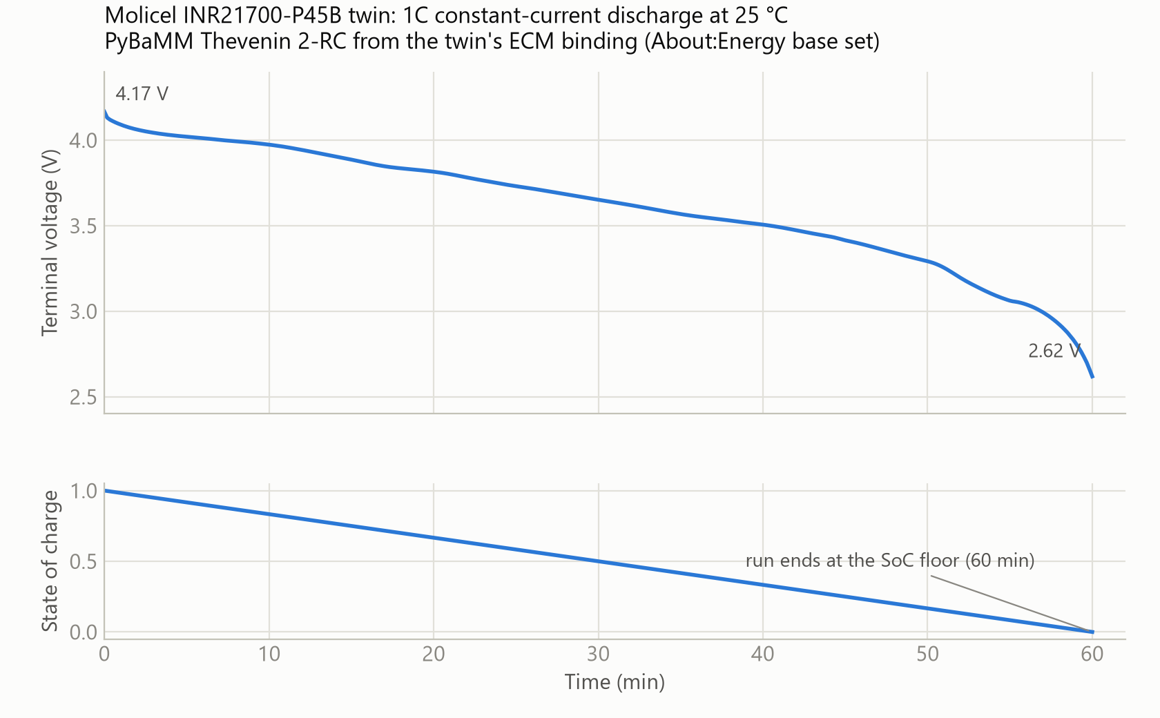
The simulated 1C discharge: terminal voltage (top) and state of charge (bottom), plotted from the BDF file the tutorial writes.#
6. Audit the finished history#
The simulation results were committed as version 4, with a data link to the trajectory and the end-of-run state:
$ battwin diff p45b.v3.twin.json p45b.v4.twin.json
versions: 3 -> 4
changed sections: data, state, state_history
version chain: intact (b.previous == hash(a))

$ battwin show p45b.v4.twin.json
Molicel INR2170-P45B (id: urn:bte:molicel-inr2170-p45b:2026-08-10)
  BTE 0.1.1 | version 4 <- sha256:85934980543...
  battinfo record: https://w3id.org/battinfo/spec/ycek-4qa3-d4v3-rm6r
  models: p45b-2rc-ecm (About:Energy base set) [custom]
  state (2026-08-10): SoC 0%
  data links: 1
Note state_history in the changed sections: the fresh-cell snapshot from the previous tutorial was not overwritten, it moved into history. The twin now carries its full trajectory.
7. What you just demonstrated#
The twin now spans registry record → identity → bench state → open ECM → simulated state, in four immutable documents, each content-hashed against the last. Every ingredient is open: the BattINFO record, the CC-BY parameter set, the ECM-PS format, PyBaMM, and the envelope itself. Anyone you hand the four files to can re-verify the chain with battwin diff, re-run the model with battwin.sim, or load the whole thing into tooling that has never heard of Python, via the published contracts.
But a simulation is only a claim. In the final tutorial the twin meets the lab: you will link the measured discharge behind this very parameter set, estimate the cell’s health from it, and let the twin quantify how well its model matches reality: Link measured data to the twin.